Tutorial 02: Backtest Validation

Overview

Item	Description
Goal	Read backtest output and risk metrics; identify overfitting, look-ahead bias, and data issues
Estimated time	60–90 minutes
Prerequisites	Tutorial 00, Tutorial 01; see Report Format Guide for the full metric table

Deep dive into backtest results, interpret reports and charts, and determine whether a strategy is truly effective.

Further reading: FAQ (blank HTML, JSON field troubleshooting, etc.).

---

Table of Contents

1. What Is a Backtest?
2. What a Backtest Tells You
3. 2.1 Report Examples in the Repository (reports/)
4. 2.2 How Do Different Strategies' Backtest Reports Look?
5. Interpreting the Backtest Report
6. Interpreting Charts
7. Risk and Attribution Analysis
8. Determining Whether a Strategy Is Effective
9. Common Backtesting Pitfalls
10. Portfolio Backtesting
11. Next Steps

---

1. What Is a Backtest?

Backtesting is "replaying" your trading strategy against historical data to see what would have happened if you had actually traded according to the strategy at the time.

Your strategy rules
     +
Historical market data
     ↓
Backtest engine → Simulated trades → Trade log + Portfolio equity curve

What a Backtest Does

• Validate ideas: Does the strategy you think works actually make money?
• Discover flaws: Are there edge cases you haven't considered?
• Parameter selection: Which parameter combination is more reasonable?
• Build confidence: Get a quantitative assessment before risking real capital

What a Backtest Cannot Tell You

• Guaranteed future profits: Historical performance does not equal future returns
• Exact profit amounts: Backtests have various biases (slippage, liquidity, etc.)
• Universal effectiveness: A strategy that works in a bull market may fail in a bear market

---

2. What a Backtest Tells You

After running a backtest, you'll get a set of core metrics:

Metric	Meaning	Benchmark
Total Return	Total profit/loss percentage over the backtest period	Beating the benchmark (CSI 300) is good
Annualized Return	Return annualized to a per-year rate	> 10% is acceptable, > 20% is excellent
Annualized Volatility	Magnitude of return fluctuations	Lower is better (< 25% preferred)
Sharpe Ratio	Excess return per unit of risk taken	> 1 is good, > 2 is excellent
Max Drawdown	Largest peak-to-trough decline	Smaller is better (< 15% preferred)
Sortino Ratio	Like Sharpe, but only considers downside volatility	> 1 is good
Alpha	Excess return over the benchmark	Positive is good
Beta	Sensitivity to the broad market	Close to 1 = tracks the market
Win Rate	May refer to "daily win rate" or "trade win rate" in the HTML, which have different meanings	See below and Report Format Guide

Note: analyze_returns returns win_rate_daily (percentage of profitable trading days) and win_rate_trade (percentage of profitable round-trip trades). You cannot directly compare these two numbers to judge strategy quality.

---

2.1 Report Examples in the Repository (reports/)

A real backtest writes four sets of files (.html / .png / .md / .json) under the repository root's reports/ directory. Filenames include timestamps; those with suffixes (e.g., _19_localdata) typically correspond to a report_suffix or script description in the example scripts.

Recommended reading: The repository's reports/README.md lists a mapping table for the example scripts. The HTML screenshot below and backtest_20260511_234245_19_localdata.html are from the same run (example 06_local_data.py); a copy is placed in assets/tutorials/ for easy display on the web — when studying locally, open the corresponding .html file in your browser alongside the Report Format Guide.

You can also open from the same result set:

• ../reports/backtest_20260511_234245_19_localdata.html (under the repo root's reports/, interactive report; the cumulative return and drawdown charts include both CSI 300 and SSE Composite dual benchmarks)
• If you haven't generated it yet: run python examples/06_local_data.py in the repo root, then find the latest *_19_localdata.* in reports/.

The abstract "strategy vs benchmark" line chart is still available at: ../assets/tutorials/sample_equity_vs_benchmark.svg.

Cross-referencing the HTML header and metric card readings: After opening the .html file mentioned above, follow Report Format Guide Section 2.8 to cross-reference each item (same source as the HTML screenshot above); if the chart area is blank, it's likely due to CDN blocking — see the FAQ.

---

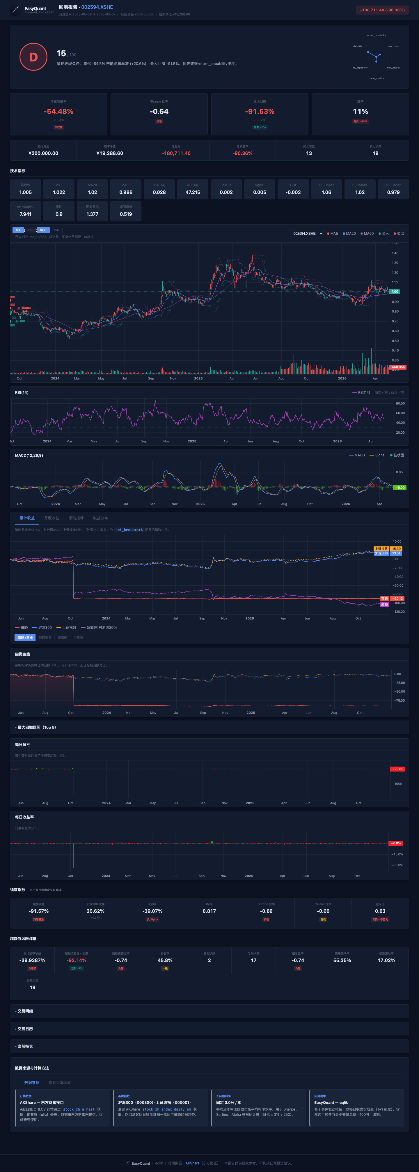
2.2 How Do Different Strategies' Backtest Reports Look?

Within the same framework, reports from different strategies have the same structure but different numbers. Below are 6 completed examples: open each script's corresponding .html to see identical page layouts with vastly different metric card values.

Note: The numbers below are from specific backtest periods and stock selections. Results will vary significantly depending on market conditions, time period, and stock selection. These are for illustration only and do not constitute investment advice.

Bollinger Bands Mean Reversion (Example 15, stock 601088 China Shenhua)

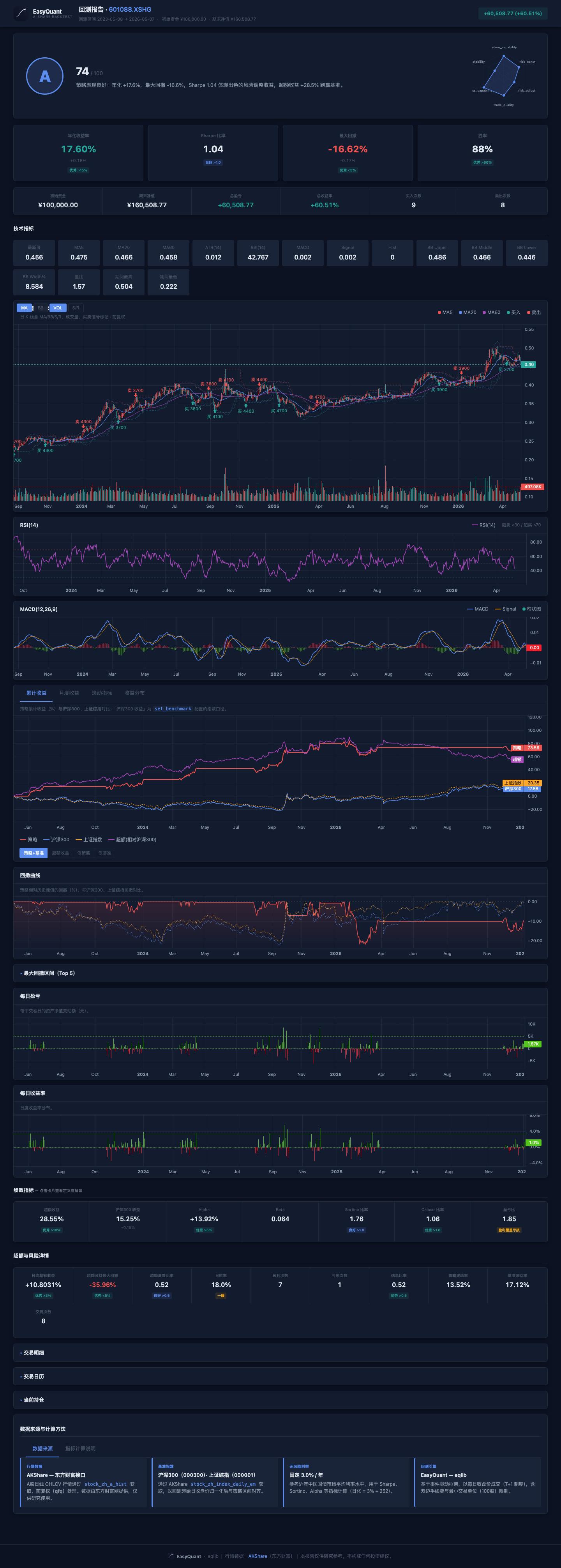
The Bollinger Bands strategy excels in range-bound markets — buy when price touches the lower band, sell at the upper band, a natural buy-low-sell-high logic. Actual backtest results will vary with market conditions.

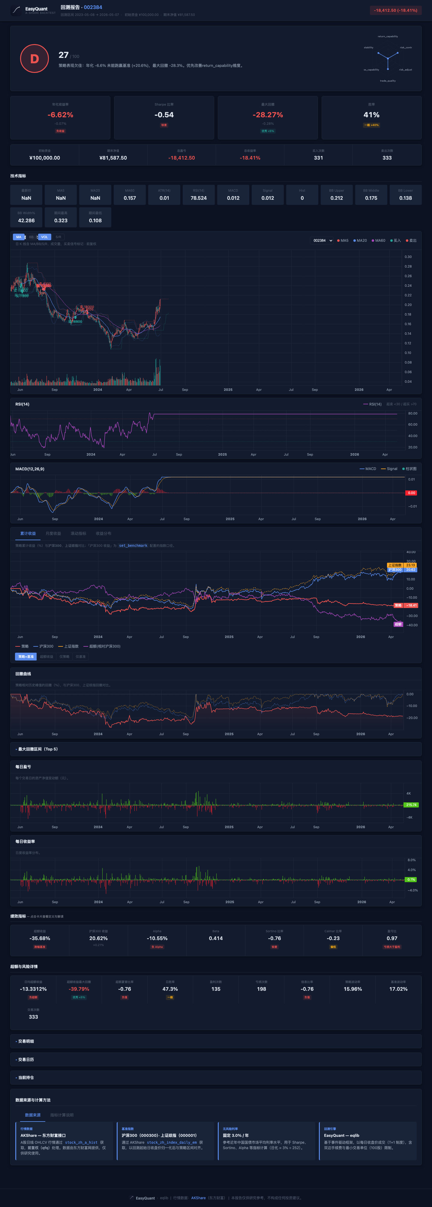
MACD Trend + Volume Confirmation (Example 16, stock 600536 China Software)

Tech stocks are highly volatile; a MACD golden cross confirmed by rising volume effectively captures trend initiation points. Actual backtest results will vary with market conditions.

Grid Trading (Example 18, stock 601857 PetroChina)

Grid trading suits low-volatility stocks with clear price ranges — repeatedly "buying low and selling high" within the range. Actual backtest results will vary with market conditions.

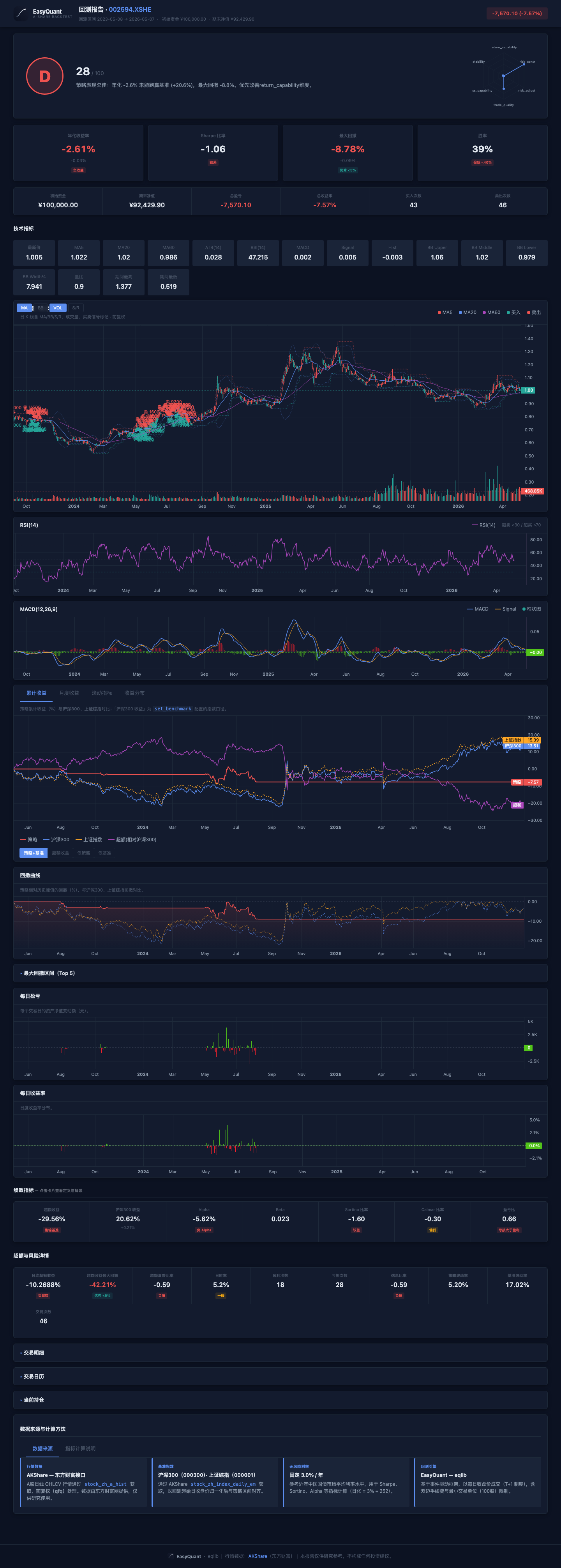
Multi-Factor Stock Selection (Example 17, 10-stock universe)

The multi-factor model selects the top 3 stocks each week from a pool of 10 based on composite momentum/volume/volatility scores, with high turnover. Actual backtest results will vary with market conditions.

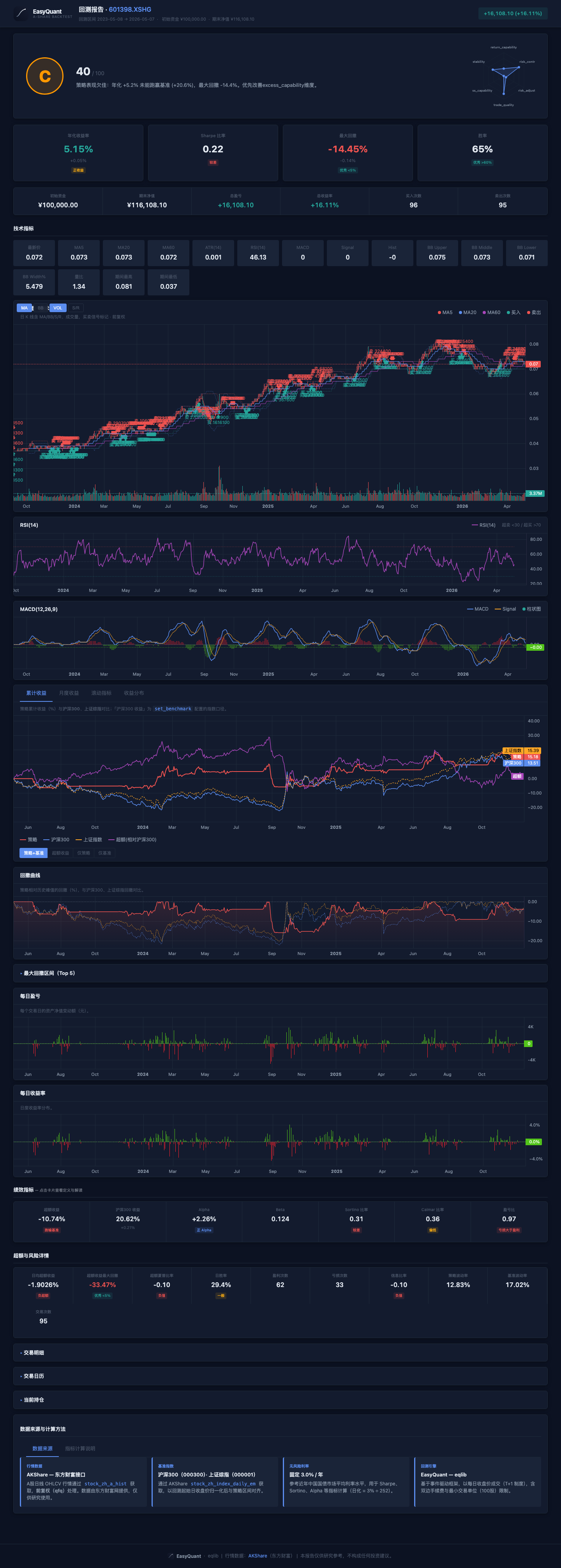
Stock Selection Strategy Interface (Example 10, 14-stock universe)

Selection based on low PE valuation + monthly rebalancing, held through the end of the period. Actual backtest results will vary with market conditions.

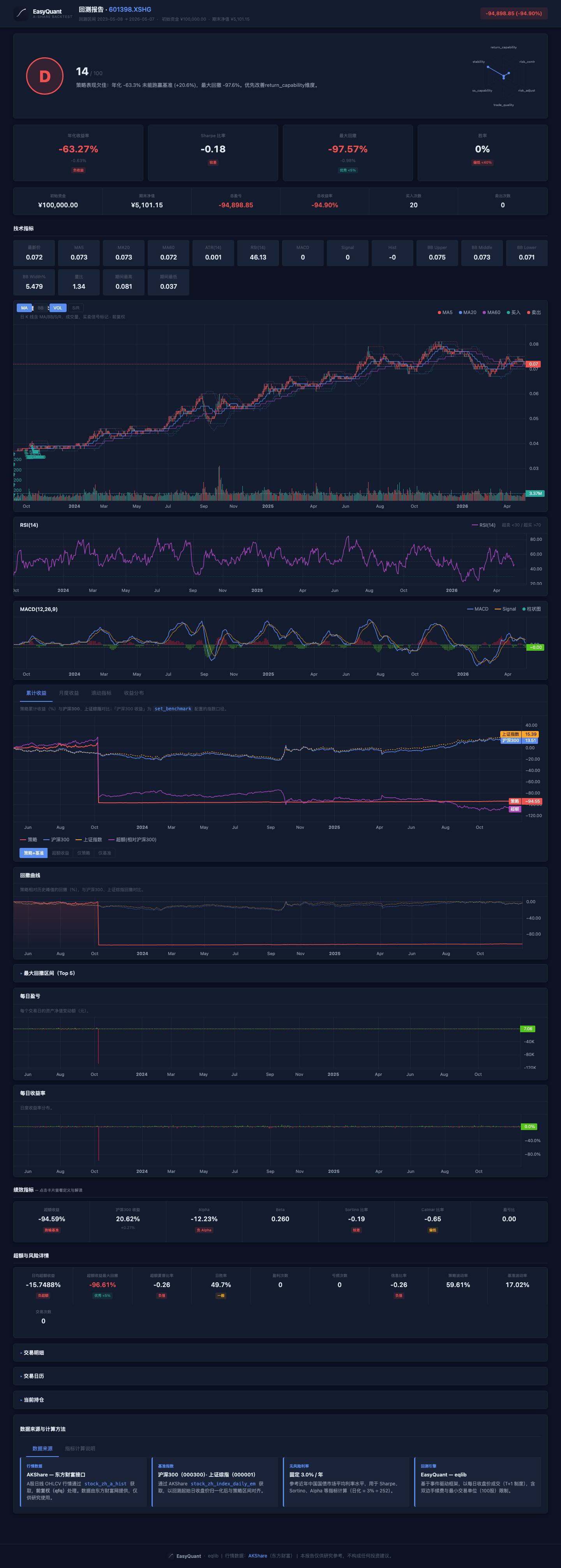
Portfolio Backtest (Example 11, 5 stocks equal-weight)

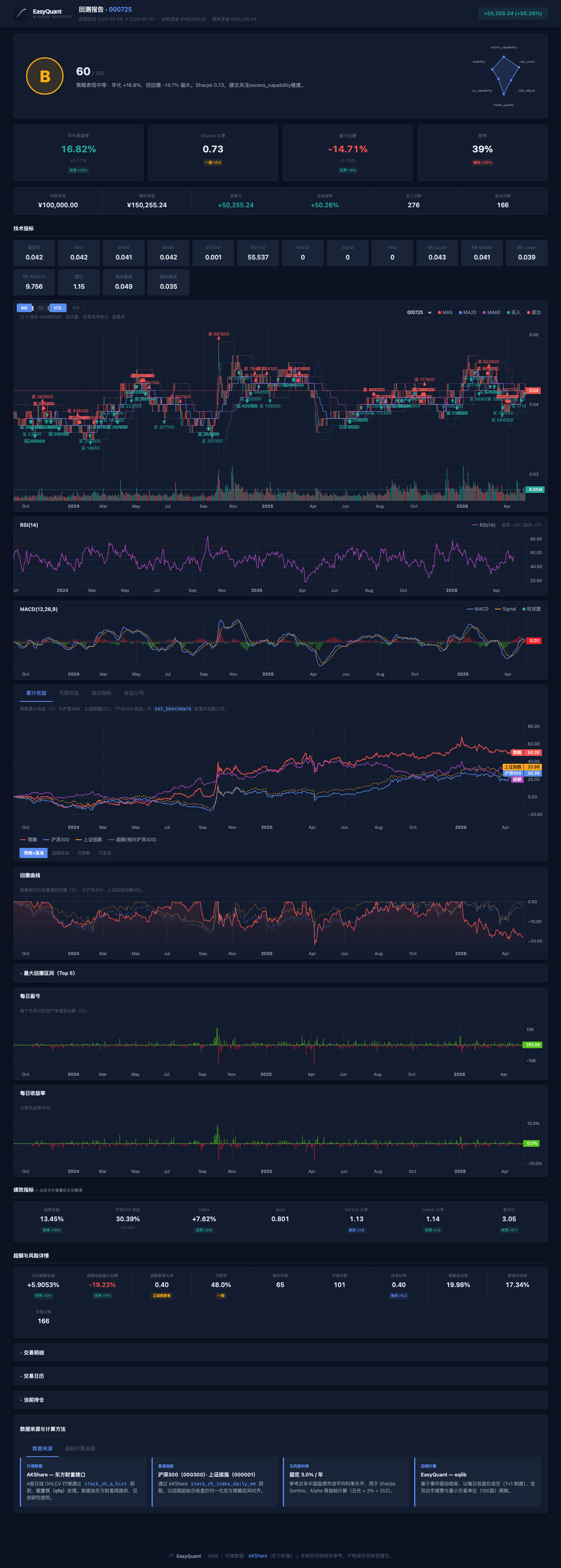
The momentum strategy's performance varies significantly depending on market regime — it may perform well in trending markets but poorly in ranging ones. Actual backtest results will vary with market conditions.

Reading suggestion: Open each corresponding .html file in your browser (see reports/README.md), and observe how the same page structure presents different metric cards, candlestick charts, drawdown curves, and trade tables across strategies.

---

3. Interpreting the Backtest Report

3.1 Running a Backtest to Generate a Report

from eqlib import *

def initialize(context):
    g.security = '601390'
    set_benchmark('000300.XSHG')
    set_order_cost(OrderCost(
        open_tax=0, close_tax=0.0005,
        open_commission=0.00025, close_commission=0.00025,
        min_commission=5,
    ))
    run_daily(market_open, time='every_bar')

def market_open(context):
    hist = attribute_history(g.security, 25, '1d', ['close'])
    if hist.empty or len(hist) < 20:
        return
    ma5 = hist['close'].tail(5).mean()
    ma20 = hist['close'].mean()
    price = hist['close'].iloc[-1]

    if price > ma5 > ma20:
        if g.security not in context.portfolio.positions:
            order_value(g.security, context.portfolio.available_cash)
            log.info('BUY %s @ %.3f' % (g.security, price))
    elif price < ma5 < ma20:
        if g.security in context.portfolio.positions:
            order_target(g.security, 0)
            log.info('SELL %s @ %.3f' % (g.security, price))

    record(price=price, ma5=ma5, ma20=ma20)

result = run_strategy(
    initialize,
    start_date='2024-01-01',
    end_date='2024-12-31',
    starting_cash=100000,
    benchmark='000300.XSHG',
    securities=['601390'],
)

3.2 Interactive HTML Report

Open reports/backtest_*.html in your browser (no local web server needed). From top to bottom, it typically includes: Summary → Metric Cards (annualized return, Sharpe ratio, max drawdown, Alpha/Beta, etc. — click for tooltips) → Candlestick & Technical Indicators → Cumulative Returns (strategy vs benchmark) → Drawdown → Daily P&L / Daily Returns → Trades, Positions tabs.

The mapping between each field and the analyze_returns dictionary keys is detailed in the Report Format Guide. The repository includes an example export index for cross-referencing real HTML/PNG: reports/README.md.

3.3 Markdown Report

File path: reports/backtest_YYYYMMDD_HHMMSS.md

# Backtest Report: 601390

## Summary
- **Period**: 2024-01-01 to 2024-12-31
- **Initial Capital**: 100,000.00
- **Final Value**: 108,234.56
- **P&L**: +8,234.56 (+8.23%)
- **Buy Orders**: 6
- **Sell Orders**: 5

## Trade Log
| # | Date | Action | Security | Price | Amount | Commission |
|---|------|--------|----------|-------|--------|------------|
| 1 | 2024-01-15 | BUY | 601390 | 4.850 | 20,618 | 29.80 |
| 2 | 2024-03-20 | SELL | 601390 | 5.120 | 20,618 | 31.75 |
| 3 | 2024-04-10 | BUY | 601390 | 5.050 | 20,500 | 29.62 |
...

Key areas to focus on:

1. P&L (Profit and Loss):
2. Absolute return (+8,234.56) and relative return (+8.23%)

3. Compare with the CSI 300 over the same period: if the CSI 300 gained 15% while your strategy only gained 8%, the strategy underperformed the benchmark

4. Trading frequency:

5. 6 buys, 5 sells → 11 total trades
6. Too many trades = high turnover = commissions eating into profits

7. Too few trades = signals may not be responsive enough

8. Per-trade P&L:

9. Review each buy and sell price trade by trade

10. If most trades are losing, the signal quality is poor

11. Commission costs:

12. Check the commission ratio for each trade
13. Small trades may have disproportionately high commission costs (due to the 5 CNY minimum)

3.4 JSON Report

File path: reports/backtest_YYYYMMDD_HHMMSS.json

import json

with open('reports/backtest_20260503_143000.json') as f:
    report = json.load(f)

# Basic metrics
print("Total return: %.2f%%" % report['pnl_pct'])
print("Number of trades:", report['num_trades'])

# Daily portfolio value curve
for entry in report['portfolio_values']:
    print(entry['date'], entry['value'])

# Custom recorded values (written via record())
for entry in report['recorded_values']:
    print(entry['date'], entry['price'], entry['ma5'])

The JSON report is suitable for further data analysis, such as: - Calculating maximum consecutive losing days - Analyzing the ratio of days in-position vs out-of-position - Plotting the cumulative return curve

3.5 HTML Interactive Report — Layer-by-Layer Guide

The HTML report is the most critical backtest analysis tool. After opening it in a browser, it is organized from top to bottom in the following layers:

Layer 1: Header Summary

The top of the page displays the backtest target, date range, initial capital, and the final asset P&L amount and percentage. This is where you judge strategy profitability at a glance.

Focus: Is P&L positive? What is the profit relative to initial capital?

Layer 2: Summary Cards

Below the header, a row of small cards shows the most critical strategy metrics:

Card	Meaning	Good Value
Annualized Return	Compound annual growth rate	> 10% acceptable, > 20% excellent
Excess Return	Strategy return − Benchmark return	Positive = outperformed the market
Sharpe Ratio	Excess return per unit of risk	> 1 good, > 2 excellent
Max Drawdown	Largest peak-to-trough decline	< 15% good, < 20% acceptable
Win Rate (Trade)	Percentage of profitable round-trip trades	> 50% good
Calmar Ratio	Annualized return / |max drawdown|	> 1 good

Focus: Don't just look at returns! The Sharpe ratio and max drawdown tell you "how much risk was taken to earn this return."

Layer 3: Detailed Metric Row

Below the summary cards, a more detailed metric row includes:

Metric	Meaning	How to Read
Annualized Volatility	Standard deviation of returns (annualized)	Lower = more stable
Sortino Ratio	Risk-adjusted return considering only downside risk	More conservative than Sharpe
Alpha	Excess return unexplained by the market	Positive = genuine alpha
Beta	Sensitivity to the broad market	1 = in sync, >1 = more aggressive
Information Ratio	Active return / tracking error	> 0.5 good
Daily Win Rate	Percentage of profitable trading days	Note: different meaning from trade win rate
Profit/Loss Ratio	Average profit / average loss	> 1.5 good

Focus: Positive Alpha + Beta near 1 means the strategy truly generates excess return, not just leveraging up or betting on direction.

Layer 4: Candlestick & Technical Indicator Chart

The strategy's price chart typically includes: - Main chart: Price line + moving averages (MA5/MA20) + buy/sell markers - Volume: Bar chart below - Green shading: Periods when a position was held

How to read: 1. Are buy/sell points reasonable? (buys at lows, sells at highs) 2. Did the price rise during holding periods? 3. Is trading frequency reasonable? (too dense may indicate overtrading)

Layer 5: Cumulative Returns

Strategy cumulative return curve vs benchmark index curve. Key comparison: Is the strategy line above the benchmark line?

• Strategy line consistently above benchmark → Strategy steadily outperforms
• Strategy line drops significantly below benchmark during some period → Strategy failed during that period
• Both lines nearly parallel → Strategy merely tracked the market, no alpha

Layer 6: Drawdown Curve

Shows the depth of the portfolio's decline from its historical high. Focus on the deepest point: Could you have tolerated that period?

Layer 7: Daily P&L / Returns

Bar chart showing daily profit/loss. Look for: - Consecutive losing days - Whether losing-day bars are longer than winning-day bars (single losses too large) - Whether returns are concentrated in just a few days

Layer 8: Tabs (Trades, Positions, etc.)

• Trades Tab: Time, price, quantity, and commission for each trade. Review trade by trade for reasonableness.
• Positions Tab: Position state at the end of the backtest.
• Attribution Tab: Brinson attribution (allocation effect, selection effect, interaction effect).

Recommended reading flow: 1. Header → Did it make money? 2. Metric cards → Sharpe > 1? Drawdown < 20%? 3. Cumulative return chart → Did it beat the benchmark? 4. Drawdown curve → Can you accept the worst case? 5. Trade table → Is each trade reasonable? 6. Attribution → Did returns come from allocation or selection?

---

4. Interpreting Charts

4.1 Chart Structure

  |                                                     |  Portfolio Value
P |  ---MA5                                              |
r |  ---MA20                                             |
i |  ---Close                                            |
c |                                                      |
e |     [SELL]    [BUY]                                  |
  |    o          o     o[SELL]                          |
  |   / \  ===== / \___/   \                             |
  |  /   \      /           \                            |
  | /     \====/             \=====                      |
  +------------------------------------------------------|-> Date

4.2 Chart Elements

Element	Meaning
Gray line	Daily closing price of the stock
Blue line	5-day moving average (short-term trend)
Orange line	20-day moving average (medium-term trend)
Green circle	Buy point (annotated below price)
Red circle	Sell point (annotated above price)
Green shading	Periods when a position was held
Green line (right axis)	Total portfolio asset value

4.3 How to Read the Chart

Good signals: - BUY points are typically at price lows (near a golden cross of moving averages) - SELL points are typically at price highs (near a death cross of moving averages) - The equity curve (right axis) trends upward overall - Price shows a clear rise during holding periods (green shading)

Bad signals: - BUY and SELL alternate frequently → Repeatedly "whipsawed" in a range-bound market - Equity curve trends steadily downward → Strategy is losing money - No significant price change during holding periods → Ineffective signals

---

5. Risk and Attribution Analysis

5.1 Comprehensive Risk Metrics

from eqlib import analyze_returns

metrics = analyze_returns(result, risk_free_rate=0.03)

print("Annualized return:    %.2f%%" % (metrics['annual_return'] * 100))
print("Annualized volatility: %.2f%%" % (metrics['annual_volatility'] * 100))
print("Sharpe ratio:          %.2f" % metrics['sharpe_ratio'])
print("Sortino ratio:         %.2f" % metrics['sortino_ratio'])
print("Max drawdown:          %.2f%%" % (metrics['max_drawdown'] * 100))
print("Calmar ratio:          %.2f" % metrics['calmar_ratio'])
print("Alpha:                 %.4f" % metrics['alpha'])
print("Beta:                  %.3f" % metrics['beta'])
print("Daily win rate:        %.2f%%" % (metrics['win_rate'] * 100))

5.2 Brinson Attribution (Multi-Stock Portfolios)

Decomposes returns into three sources:

from eqlib import brinson_attribution

attr = brinson_attribution(result)

print("Allocation effect: %.4f  <-- Returns from asset allocation (sector/industry selection)" % attr['allocation_effect'])
print("Selection effect:  %.4f  <-- Returns from individual stock selection" % attr['selection_effect'])
print("Interaction effect: %.4f  <-- Combined effect of allocation and selection" % attr['interaction_effect'])

• Allocation effect > 0: Your sector/industry choices were correct
• Selection effect > 0: Your stock picks within each sector were correct
• Interaction effect: Usually a small adjustment term

5.3 Simplified Factor Analysis

from eqlib import simple_factor_analysis

ff = simple_factor_analysis(result)

print("Market Beta:           %.3f  <-- Market sensitivity" % ff['market_beta'])
print("Annualized Alpha:      %.4f  <-- Excess return unexplained by market" % ff['alpha_annual'])
print("Momentum correlation:  %.3f" % ff['momentum_correlation'])
print("Residual volatility:   %.3f" % ff['residual_volatility'])

Note: fama_french_analysis has been deprecated; use simple_factor_analysis instead.

---

6. Determining Whether a Strategy Is Effective

6.1 Core Evaluation Criteria

Question	Criterion
Does the strategy make money?	Total return > 0
Does it beat the market?	Strategy return > Benchmark return (CSI 300)
Is risk-adjusted performance good?	Sharpe ratio > 1
Is the max drawdown acceptable?	Max drawdown < your risk tolerance
Is trading frequency reasonable?	Not daily turnover, nor once every six months

6.2 Comprehensive Evaluation Template

metrics = analyze_returns(result, risk_free_rate=0.03)

checks = []
checks.append(("Return > 0", metrics['total_return'] > 0))
checks.append(("Beat benchmark", metrics['alpha'] > 0))
checks.append(("Sharpe > 1", metrics['sharpe_ratio'] > 1))
checks.append(("Drawdown < 20%", abs(metrics['max_drawdown']) < 0.20))
checks.append(("Win rate > 50%", metrics['win_rate'] > 0.50))

print("--- Strategy Evaluation ---")
passed = 0
for name, ok in checks:
    status = "PASS" if ok else "FAIL"
    if ok:
        passed += 1
    print("  [%s] %s" % (status, name))
print("Passed %d/%d checks" % (passed, len(checks)))

6.3 Out-of-Sample Validation

# Training set: 2020-2023, used for parameter tuning
result_train = run_strategy(
    initialize, '2020-01-01', '2023-12-31',
    starting_cash=100000, securities=['601390'],
)

# Test set: 2024, used for validation
result_test = run_strategy(
    initialize, '2024-01-01', '2024-12-31',
    starting_cash=100000, securities=['601390'],
)

# If training Sharpe = 2.0, test Sharpe = 0.3 -> overfitting
# If training Sharpe = 1.5, test Sharpe = 1.2 -> parameters are stable

---

7. Common Backtesting Pitfalls

7.1 Overfitting

Backtest annualized 50%, live annualized 5%
Cause: Parameters were repeatedly tweaked on historical data, effectively "memorizing" past price movements

How to identify: Results change drastically with minor parameter tweaks → overfitting

7.2 Look-Ahead Bias

# Wrong example: using today's closing price for an open-market decision
# attribute_history returns yesterday's data — this is correct
# But if the strategy uses get_today_close() or any method that includes today's data,
# that constitutes look-ahead bias

7.3 Survivorship Bias

Only tested stocks that are still listed → Ignored delisted / ST (Special Treatment) stocks
→ Backtest results are artificially inflated

7.4 Ignoring Liquidity

Backtest buys 1M CNY of a stock, but the stock's average daily volume is only 500K
→ Impossible to fill in reality, backtest results are invalid

7.5 Backtest Period Too Short

Only backtested 3 months → May have coincided with a bull/bear market
→ Recommend at least 1-2 years, covering different market environments

---

8. Portfolio Backtesting

8.1 Single Stock vs Portfolio

	Single-Stock Backtest	Portfolio Backtest
Use case	Validate a single strategy logic	Multi-stock rotation, asset allocation
API	run_strategy / run_backtest	run_portfolio_backtest
Stock universe	One stock	Multiple stocks
Position sizing	context.portfolio.available_cash	position_pct or position_amount

8.2 Portfolio Backtest Example

from eqlib import StrategyConfig, run_portfolio_backtest

# Define configuration
config = StrategyConfig(
    starting_cash=200000,
    securities=['601390', '600519', '000858'],
    benchmark='000300.XSHG',
    position_pct=0.33,       # Each stock uses at most 33% of available cash
    start_date='2024-01-01',
    end_date='2024-12-31',
    report_suffix='multi_stock_v1',
)

# Strategy function
def my_strategy(context):
    for sec in context.universe:
        hist = attribute_history(sec, 25, '1d', ['close'])
        if hist.empty:
            continue
        ma20 = hist['close'].tail(20).mean()
        price = hist['close'].iloc[-1]

        if price > ma20 * 1.02:
            order_value(sec, context.portfolio.available_cash * 0.33)
        elif price < ma20 * 0.98 and context.portfolio.positions.get(sec):
            order_target(sec, 0)

# Run the backtest
result = run_portfolio_backtest(config, my_strategy)

8.3 Portfolio Backtest Output

==================================================
Portfolio Backtest: 2024-01-01 → 2024-12-31
Universe: ['601390', '600519', '000858']
==================================================
Starting Cash:         200,000.00
Final Value:           215,342.00
P&L:                 +15,342.00 (+7.67%)
Total Trades:              12

--- Per-Stock Summary ---
  600519: 3 buys, 3 sells, net shares 0, realized ¥5,200.00
  601390: 4 buys, 4 sells, net shares 0, realized ¥3,100.00
  000858: 5 buys, 5 sells, net shares 0, realized ¥7,042.00

---

9. Next Steps

After learning to interpret backtest results, here's what's next:

• Tutorial 03: Strategy Optimization & Improvement — Parameter tuning, portfolio optimization, attribution analysis, avoiding overfitting
• Tutorial 05: RSI Mean Reversion Strategy — Switch to a different strategy approach: mean reversion
• Example 20: Support/Resistance Portfolio Strategy — A complete multi-stock portfolio strategy case study with pre-generated backtest reports for direct review
• Tutorial 04: Paper Trading to Live Trading — From paper trading to PTrade/QMT live deployment