Tutorial 00: Environment Setup & Quantitative Fundamentals¶
Overview
| Item | Description |
|---|---|
| Goal | Set up your Python environment, install eqlib, run a backtest, and open the HTML report in your browser |
| Estimated time | ~30 minutes |
| Prerequisites | None (complete beginners can start with the prerequisite links below) |
Before reading the quantitative fundamentals in order, complete this section first: ensure your Python environment and
eqlibare set up and a backtest runs successfully, so later tutorial code won't fail.
No Python background? Read Prerequisites: Python Basics & Environment Setup. Unfamiliar with technical indicators? Read Prerequisites: Technical Analysis Fundamentals. Not familiar with A-share rules? Read Prerequisites: A-Share Market Fundamentals.
1. What Environment Do You Need?¶
| Item | Requirement |
|---|---|
| Python | 3.10, 3.11, or 3.12 (eqlib declares requires-python >= 3.10 in pyproject.toml) |
| OS | macOS / Linux / Windows — all supported |
| Network | Initial market data fetch uses akshare online APIs; internet access (or access to the data source) is required |
2. Installing eqlib (Recommended)¶
Run the following from the repository root directory (this also installs dependencies such as akshare, pandas, etc.):
cd EasyQuant
python3 -m venv .venv          # Optional but strongly recommended
source .venv/bin/activate    # Windows: .venv\Scripts\activate

# Option 1: Install from source (from the repo root)
pip install .
# For development/debugging: pip install -e .

# Option 2: Install from PyPI (no need to clone the repo)
# pip install easyquant-eqlib
Verify:
If pip install . fails, check the FAQ section on "Installation & Environment" first.
3. Running Your First Example Backtest¶
From the repository root, run:
The script will download (or update) data and run the backtest. When finished, the terminal will print the paths to PNG, HTML, Markdown, and JSON files under reports/.
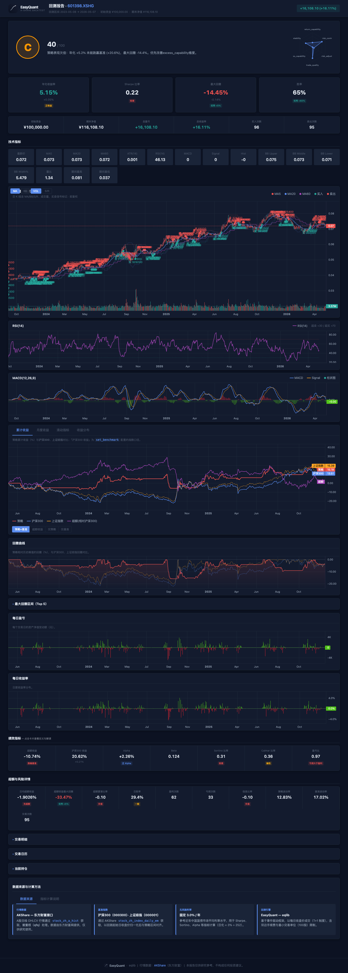
Open the .html file in your browser and scroll from top to bottom: metric cards → charts → fills and positions. Field descriptions can be found in Report & Metrics Reference.
To compare with the saved example outputs in reports/, see reports/README.md (recommended to read alongside example_report_html_19_localdata.png and the Tutorial 02 illustrations).
4. Optional: Test the Data API Only¶
If you want to verify your network connection and data availability first, run:
This script focuses on demonstrating data APIs such as get_price and fetch_stock_data — it does not produce a full backtest report.
5. Recommended: Pre-download Target Stocks Locally, Then Run a Quick Backtest¶
If you already know which stocks you want to study, download the data locally first and then use use_local=True for faster backtests. This significantly reduces network-related variability.
python - <<'PY'
from eqlib import set_local_data_dir, save_stock_local, list_local_stocks

set_local_data_dir('/home/user/eqlib_data')  # Absolute path recommended for reuse across projects
targets = ['601390', '600519', '000858', '000300.XSHG']  # Including benchmark

for sec in targets:
    path = save_stock_local(sec, start_date='2020-01-01', end_date='2024-12-31')
    print(sec, '->', path)

print('local files:', list_local_stocks())
PY
Then enable local mode when running any backtest script:
result = run_strategy(
    initialize,
    start_date='2024-01-01',
    end_date='2024-12-31',
    securities=['601390'],
    use_local=True,
)
It is recommended to run examples/06_local_data.py first to validate the offline workflow.
Tip: The date range of your locally downloaded data should cover your backtest period. If the backtest dates extend beyond the local file range, download the missing data first.
See more API details at:
6. How Do Tutorials, Examples, and the Formal Documentation Fit Together?¶
| Resource | Purpose |
|---|---|
docs/tutorials/ (this directory) |
Topic-by-topic, progressive learning: why things are done this way, common pitfalls |
examples/ |
Runnable scripts you can copy — see the Examples.md index |
docs/README.md |
Documentation hub: entry point for the user manual, full API table, FAQ, and report interpretation |
7. Next Steps¶
Once you can successfully run examples/03_run_backtest.py and open the HTML report, continue with the quantitative trading fundamentals below, then move on to:
Quantitative Trading Fundamentals¶
Understand quantitative trading from scratch — learn the core concepts of strategy development and key considerations.
| Item | Description |
|---|---|
| Goal | Build a foundational understanding of quantitative trading and strategy development; learn the full workflow and common pitfalls |
| Estimated time | 45–60 minutes (feel free to skim by section) |
| Prerequisites | Complete the environment setup and first run above |
1. What Is Quantitative Trading?¶
Quantitative trading is an approach that uses mathematical models and computer programs to formulate and execute trading decisions. Unlike discretionary trading (based on experience and intuition), quantitative trading codifies investment logic into explicit rules that a computer executes automatically.
1.1 A Simple Example¶
Discretionary trading idea:
"ICBC has been going up lately and the moving averages look like they're about to cross — let me buy some and see."
Quantitative trading idea:
"When the 5-day MA of 601390 crosses above the 20-day MA, and the day's closing price is more than 2% above the 5-day MA, buy with all available cash. When the 5-day MA crosses below the 20-day MA, sell everything."
The key difference: verifiable, reproducible, auditable.
1.2 Why Python?¶
Python is the most widely used language in quantitative trading, for good reasons: - Clean syntax, low barrier to entry - The richest ecosystem of financial libraries (pandas, numpy, scipy, matplotlib) - Abundant, free data sources (akshare, tushare, etc.)
1.3 Where EasyQuant Fits¶
EasyQuant (eqlib) is a lightweight quantitative strategy framework for the China A-share market. It provides:
- A simple, intuitive strategy API (event-driven model)
- Free A-share data (akshare)
- A complete workflow: backtesting, report generation, paper trading
- Export to PTrade/QMT platforms for live trading
2. The Five Core Elements of a Quantitative Strategy¶
Every runnable quantitative strategy consists of these five elements:
2.1 Universe¶
Decide which stocks you will trade. Common approaches:
- Fixed list: preselect a handful of stocks (e.g., '601390', '600519', '000858')
- Index constituents: CSI 300, CSI 500 constituents
- Sector: stocks in a given industry (e.g., baijiu, new energy)
- Dynamic screening: real-time filtering by fundamentals (PE/PB/ROE), technicals (MA alignment), money flow, etc.
2.2 Entry Signal¶
When do you buy? This is your signal. Common types:
| Type | Example |
|---|---|
| Trend following | Short-term MA crosses above long-term MA (golden cross) |
| Mean reversion | Price deviates from the MA by more than N standard deviations — bet on reversion |
| Momentum | Top 10% stocks by return over the past N days |
| Event-driven | Earnings release, dividend, Dragon Tiger list |
| Money flow | Net institutional inflow for N consecutive days |
2.3 Exit Signal¶
When do you sell? Exits are as important as entries:
| Type | Example |
|---|---|
| Signal reversal | Buy on golden cross → sell on death cross |
| Stop-loss | Unconditional sell if loss exceeds 5% |
| Take-profit | Sell after a 20%+ gain pulls back by 5% |
| Time stop | Sell if a position has not turned profitable after 20 trading days |
| Rebalancing | Reassess periodically (e.g., every Monday) and swap for better candidates |
2.4 Position Sizing¶
How much do you buy each time?
| Method | Description | Best for |
|---|---|---|
| All-in | All capital into a single stock | Single-stock strategies |
| Equal weight | Split capital equally across stocks | Portfolio rotation |
| Fixed fraction | Invest a fixed percentage of available capital each time | Gradual position building |
| Kelly criterion | Optimal size based on win rate and payoff ratio | Mature strategies with historical data |
| ATR-based sizing | Dynamically adjust size based on volatility | Risk-controlled strategies |
2.5 Risk Management¶
- Maximum single-stock position (e.g., no more than 30% of total capital)
- Maximum drawdown threshold (pause the strategy if drawdown exceeds 15%)
- Stop-loss limit (force-sell if a single stock loses more than 8%)
- Sector concentration limit (no more than 40% in a single industry)
3. The Full Strategy Development Workflow¶
3.1 Step 1: Form an Idea¶
Ideas can come from: - Reading classic trading books (Way of the Turtle, Technical Analysis of the Financial Markets, Quantitative Investment) - Studying market anomalies (e.g., "January effect", "Monday effect") - Observing others' successful approaches - Your own trading experience and reflections
3.2 Step 2: Formalize the Rules¶
Turn a vague idea into explicit, computable rules:
Vague idea: "Low-priced stocks are more likely to go up"
Formalized:
  1. Select A-share stocks priced below 10 CNY
  2. Exclude ST stocks
  3. Buy all qualifying stocks with equal weight every Monday
  4. Sell everything every Friday
  5. Backtest period: 2023-01-01 to 2024-12-31
3.3 Step 3: Backtest¶
Run your rules against historical data to see how they perform.
What a backtest tells you: - Is the strategy profitable? What is the annualized return? - How large is the maximum drawdown? Can you tolerate it? - What is the Sharpe ratio? Is it good on a risk-adjusted basis? - Did it beat or underperform the benchmark?
3.4 Step 4: Optimize (Beware of Overfitting)¶
Tune parameters to improve performance.
But watch out for overfitting — perfect on historical data, losing money live. Ways to avoid it: - Out-of-sample validation: tune on 2020–2023, validate on 2024 - Parameter stability tests: small parameter tweaks should not cause dramatic result changes - Limit the number of parameters: more parameters = higher overfitting risk - Logic-driven, not data-driven: parameters should be grounded in economics or behavioral finance
3.5 Step 5: Paper Trading¶
Once the backtest passes, run a paper trade on live market data — validate the strategy in a "real" environment without risking real capital.
3.6 Step 6: Live Trading¶
After paper trading validates the strategy, start live trading with a small position and gradually scale up.
4. Ten Common Beginner Mistakes¶
4.1 Ignoring Transaction Costs¶
# Wrong: not accounting for commissions
# 5 trades/day × (0.025% commission + 0.05% stamp duty) = huge cumulative drag over a year

# Correct: set realistic transaction costs
set_order_cost(OrderCost(
    open_tax=0,
    close_tax=0.0005,          # 0.05% stamp duty (halved since Aug 2023)
    open_commission=0.00025,   # 0.025% commission on buy
    close_commission=0.00025,
    min_commission=5,         # Minimum commission: 5 CNY
))
4.2 Look-ahead Bias¶
# Wrong: using today's closing price to make a decision that is executed at open
def market_open(context):
    # Getting today's close at open — impossible!
    today_close = get_today_close('601390')
    if today_close > ma20:
        order(...)

# Correct: only use historical data
def market_open(context):
    # Use yesterday's data and earlier
    hist = attribute_history('601390', 20, '1d', ['close'])
    # hist contains only the 20 days up to and including yesterday
4.3 Survivorship Bias¶
# Wrong: only backtesting on currently listed stocks, ignoring delisted/ST stocks
# This inflates backtest results

# Correct: use historical constituent lists, or scan_market to get the full market at the time
4.4 Ignoring Liquidity¶
# Wrong: backtesting large orders on low-cap stocks — actual volume can't support it
# Daily volume is 1M CNY, but your backtest tries to buy 5M — impossible to fill

# Correct: check average daily volume and ensure your order size is reasonable
vol = attribute_history(sec, 20, '1d', ['volume'])
avg_volume = vol['volume'].mean()
# Your order should not exceed 5–10% of average daily volume
4.5 Overfitting (Over-optimization)¶
# Wrong: tweaking parameters endlessly until the equity curve looks perfect
# MA5/MA20 doesn't work → try MA7/MA23 → try MA3/MA17 → ...
# Eventually you find a parameter set that gives 50% annualized in backtest —
# but will likely lose money live

# Correct:
# 1. Parameters should have a logical rationale (why 20 and not 23?)
# 2. Test parameter stability (MA18/MA22 and MA20/MA25 should yield similar results)
# 3. Reserve out-of-sample data for final validation
4.6 Ignoring Slippage¶
# Wrong: assuming you can trade at the closing price
# By the time your order reaches the market, the price may have moved

# How EasyQuant handles it:
# Orders are queued during the callback and filled at the next trading day's open.
# In live trading, slippage of 0.1%–0.3% is typical.
4.7 Forgetting the A-Share T+1 Rule¶
# Wrong: buying today and trying to sell today
# A-shares operate on T+1: stocks bought today can only be sold on the next trading day

# EasyQuant handles T+1 automatically internally
# via Position.closeable_amount, which controls the sellable quantity
4.8 Focusing Only on Returns, Ignoring Risk¶
# Wrong: Strategy A: 30% annualized, 40% max drawdown
#        Strategy B: 15% annualized, 8% max drawdown
# Choosing A based on return alone — but B may have a better Sharpe ratio

# Correct: focus on risk-adjusted metrics
# - Sharpe Ratio
# - Maximum Drawdown
# - Sortino Ratio
4.9 Not Setting a Stop-loss¶
# Wrong: having a buy signal but no sell / stop-loss rule
# "Just hold it if it drops — it'll come back eventually" — some stocks never do

# Correct: every buy signal should have a corresponding sell rule
# Signal-based stop-loss / fixed-percentage stop-loss / ATR trailing stop / time stop
4.10 Going Straight to Live Trading¶
# Wrong: running a backtest and then going all-in live immediately
# Correct:
# 1. Backtest validation (historical data)
# 2. Paper trading (live market data, virtual capital)
# 3. Small live position (real capital, controlled risk)
# 4. Gradually increase position size
5. What Knowledge Do You Need?¶
The following three prerequisite files provide more comprehensive learning material — consult them as needed:
| Prerequisite file | Topics covered | Link |
|---|---|---|
| Python Basics & Environment Setup | Syntax cheat sheet, core pandas/numpy operations, virtual environments | prerequisites/python-basics.md |
| Technical Analysis Fundamentals | OHLCV, moving averages, RSI, MACD, Bollinger Bands, ATR, KDJ, ADX | prerequisites/technical-concepts.md |
| A-Share Market Fundamentals | Stock code formats, T+1, price limits, major indices, ST stocks, fees & taxes | prerequisites/ashare-knowledge.md |
5.1 Essential (Before Writing Strategies)¶
| Area | Content | Suggested study time |
|---|---|---|
| Python basics | Variables, functions, loops, conditionals | 1–2 weeks; or consult the prerequisite file directly |
| pandas | DataFrame, Series, indexing, aggregation | 1–2 weeks; core usage in prerequisite file §4 |
| Technical indicators | Moving averages, MACD, RSI, Bollinger Bands | Learn as you go; systematic overview in the prerequisite file |
| A-share rules | T+1, price limits, transaction fees | Half a day; see the prerequisite file |
5.2 Recommended (When Deepening Strategy Optimization)¶
| Area | Content |
|---|---|
| Risk management | Kelly criterion, VaR, maximum drawdown |
| Portfolio theory | Efficient frontier, risk parity |
| Performance attribution | Brinson attribution, Fama-French factors |
| Data visualization | matplotlib basic charts |
5.3 Bonus¶
| Area | Content |
|---|---|
| Machine learning | Classification, regression, feature engineering |
| Time series analysis | ARIMA, GARCH |
| Databases | SQLite, PostgreSQL |
| Systems programming | Multiprocessing, scheduled tasks |
6. Next Steps¶
With the fundamentals covered, move on to:
- Tutorial 01: Writing Your First Strategy — Write and run your first quantitative strategy with EasyQuant
- Tutorial 02: Backtest Validation — Deep-dive into backtesting and evaluate your strategy's historical performance
- Tutorial 03: Strategy Optimization & Improvement — Parameter tuning, avoiding overfitting, combining strategies
- Tutorial 04: Paper Trading to Live Trading — From paper trading to PTrade/QMT live deployment
- Tutorial 05: RSI Mean Reversion Strategy — Deep-dive into the classic mean reversion strategy type
- Tutorial 06: Sector Rotation Strategy — Exploit A-share sector rotation dynamics for excess returns
- Tutorial 07: Multi-Factor Stock Selection — Systematically combine multiple factors to select high-quality stocks